Forecasting Asset Covariances and Variances Using 
Multi-scale Risk Models: Evidence from the Amman Stock Exchange

Said Sami Al Hallaq; Mohammad Ajlouni; Laith Abu- Alfoul

doi:doi:10.11648/j.jbed.20261101.11

Research Article |

| Peer-Reviewed

Forecasting Asset Covariances and Variances Using Multi-scale Risk Models: Evidence from the Amman Stock Exchange

Said Sami Al Hallaq^*

, Mohammad Ajlouni, Laith Abu- Alfoul

Published in Journal of Business and Economic Development (Volume 11, Issue 1)

Received: 27 October 2025 Accepted: 6 November 2025 Published: 28 February 2026

Views: Downloads:

Download PDF

Share This Article

Twitter
Linked In
Facebook

Abstract

This study aims to forecast asset variances and covariances through the application of multi-scale risk models. Using daily data for 61 firms listed on the Amman Stock Exchange (ASE) over the period from January 1, 2001, to December 31, 2015, the analysis investigates the dynamic behaviour of asset returns across different time horizons. To enhance the robustness and reliability of the findings, several econometric and statistical techniques are employed, including the CUSUM test to assess structural stability, the Granger causality test to examine predictive relationships, wavelet transformation to capture time-frequency dynamics, and unit root tests to verify stationarity properties. The multi-scale risk model serves as the principal analytical framework, allowing for a comprehensive examination of the evolving interdependencies among asset returns. The empirical results indicate that market risk premium coefficients significantly explain variations in portfolio returns, highlighting the importance of systematic risk factors in asset pricing. Furthermore, portfolios composed of lower-value stocks outperform those containing higher-value stocks, while smaller-sized portfolios consistently generate higher returns than larger-sized portfolios during the sample period. Overall, the findings demonstrate the effectiveness of multi-scale risk models in forecasting asset variances and covariances. The model exhibits strong explanatory power in capturing daily portfolio return dynamics on the ASE, thereby contributing to improved portfolio optimization strategies and more accurate risk prediction. These results underscore the practical and theoretical value of multi-scale modelling in financial risk management.

Published in	Journal of Business and Economic Development (Volume 11, Issue 1)
DOI	10.11648/j.jbed.20261101.11
Page(s)	1-15
Creative Commons	This is an Open Access article, distributed under the terms of the Creative Commons Attribution 4.0 International License (http://creativecommons.org/licenses/by/4.0/), which permits unrestricted use, distribution and reproduction in any medium or format, provided the original work is properly cited.
Copyright	Copyright © The Author(s), 2026. Published by Science Publishing Group

Keywords

Forecasting, Portfolio Variances and Covariances, Multi-scale Risk Models, Market Risk Premium, Wavelet Transform, Granger Causality Test, Unit Root Tests, Amman Stock Exchange (ASE)

1. Introduction

Investments in capital markets are inherently exposed to multiple types of risk, including loss, default, and bankruptcy. Therefore, investors continuously seek the optimal combination of assets that maximizes expected return while minimizing risk exposure. The foundations of this pursuit were established by Harry Markowitz

[34]

in his pioneering work “Portfolio Selection,” which introduced the concept of diversification and laid the groundwork for modern portfolio theory (MPT). Markowitz proposed that investors should base portfolio selection on a trade-off between risk—measured by variance—and expected return, under the assumption that investors are rational and risk-averse.

In the context of MPT, investors aim to expand their utility functions to account for both return expectations and risk tolerance. In other words, they seek to maximize returns for a given level of risk or minimize risk for a given level of return. The portfolios that successfully achieve this balance are known as optimal portfolios, which are essential for enhancing investment performance and ensuring market efficiency. Over time, portfolio theory has evolved significantly, giving rise to a range of asset pricing models designed to improve portfolio optimization through more accurate estimation of systematic risk and return dynamics.

This study contributes to that ongoing development by forecasting asset covariances and variances using multi-scale risk models to identify optimal portfolios within the Amman Stock Exchange (ASE). Recognizing the importance of precise risk forecasting for investment decisions, the study explores whether multi-scale decomposition of return series can enhance predictive performance. Specifically, it posits that variance–covariance matrices derived from decomposed return data outperform those derived from undecomposed data, offering more reliable estimates for portfolio construction.

Accordingly, the research seeks to address the following key questions: (a) Can covariance be effectively predicted through factor models? (b) Can variance–covariance matrices of different models and scales be applied to construct minimum-variance portfolios? (c) Do multi-scale risk models provide reliable forecasts of asset covariances and variances?

The main objective of this paper is to forecast asset covariances and variances using multi-scale risk models. The specific objectives are as follows: (1) To predict covariances using factor-based models. (2) To employ variance–covariance matrices from different models and scales for constructing minimum-variance portfolios. (3) To forecast asset covariances and variances to improve portfolio optimization and risk management.

The remainder of this paper is organized as follows: Section I presents the theoretical background and evolution of portfolio selection and asset pricing models, including the Capital Asset Pricing Model (CAPM), the Fama and French

[18]

Three-Factor Model, and their multi-scale and five-factor extensions. Section II provides a review of empirical studies related to forecasting asset covariances and variances in portfolio optimization. Section III describes the data and methodology used in the analysis, including model design and variable construction. Section IV reports the empirical findings and interprets the results. Section V concludes with a summary of key results and implications for investors, policymakers, and future research.

2. Theoretical and Institutional Framework

The modern theory of investment in financial assets—distinct from investment in real assets and derivatives—has evolved through three major paradigms. The first is the single-factor model derived from Modern Portfolio Theory (MPT), first introduced by Treynor

[42, 43]

and later developed by Sharpe

[40]

, Lintner

[30]

and Mossin

[36]

.in the Capital Asset Pricing Model (CAPM). The second is the Arbitrage Pricing Theory (APT) developed by Ross

[38]

, while the third encompasses multi-factor models, such as the Fama and French Three-Factor

[21]

and Five-Factor

[21]

frameworks. Systematic risk has been shown to vary across time scales, supporting the application of multi-resolution techniques in financial modeling

[22]

Modern Portfolio Theory, proposed by Harry Markowitz

[34]

in his seminal paper “Portfolio Selection,” laid the foundation for contemporary financial economics. Subsequent developments have extended Markowitz’s framework to incorporate more dynamic optimization techniques and advanced estimation procedures

[15]

. Later expanded by William Sharpe

[40]

and others, MPT provides a rigorous framework for constructing efficient investment portfolios based on maximizing expected return while minimizing risk. As emphasized by Fabozzi et al.

[17]

, MPT represents a normative theory—one that prescribes how rational investors should behave in constructing portfolios. Volatility risk has also been shown to be priced across asset classes, reinforcing the importance of incorporating dynamic risk components into asset pricing models

[13]

. Alternative coherent risk measures such as spectral risk measures have also been proposed to improve portfolio optimization under downside risk conditions

[2]

At the core of MPT lies the principle of diversification, a concept encapsulated in the classical adage “Do not put all your eggs in one basket.” By diversifying across assets with imperfect correlations, investors can reduce unsystematic risk and stabilize portfolio performance. The theory formalized the notion of the efficient frontier, representing portfolios that yield the maximum possible return for a given level of risk. Mathematically, total portfolio risk depends not only on the variance of individual asset returns but also on the covariance among asset pairs. Additional evidence suggests that consumption and cash flow risks contribute to explaining cross-sectional stock return variation

[14]

The CAPM was first introduced by Treynor

[42, 43]

and later developed by Sharpe

[40]

, Lintner

[30]

and Mossin

[36]

. The model extends MPT by linking an asset’s expected return to its systematic risk, measured by the beta coefficient (β), which captures the covariance between the asset’s return and the market return. CAPM assumes that investors are compensated only for systematic (non-diversifiable) risk, as idiosyncratic risk can be eliminated through diversification. Correlation risk has also been shown to significantly influence optimal portfolio choice decisions [10].

The relationship between Fama–French factors and intertemporal CAPM state variables has also been explored in the literature, providing further insight into the dynamic interaction between risk factors and macroeconomic innovations

[27]

Despite its foundational importance, the CAPM has faced empirical challenges. Miller and Scholes

[35]

highlighted inconsistencies in estimating expected returns due to the time variability of risk-free rates and the nonlinear relationship between beta and returns. Later, Fama and French

[18]

demonstrated that high book-to-market (value) stocks earn higher average returns than predicted by CAPM, suggesting that additional factors beyond market beta influence expected returns.

To address CAPM’s limitations, Fama and French

[19]

proposed the Three-Factor Model (FF3F), which includes two additional explanatory variables: the size risk premium (SMB – Small Minus Big), representing the excess return of small-cap over large-cap firms, and the value risk premium (HML – High Minus Low), capturing the excess return of value stocks over growth stocks. Empirical validation of asset pricing models often follows the two-pass regression approach introduced by Fama and MacBeth

[20]

. Empirical results demonstrated that these additional factors significantly improved the model’s explanatory power, reducing pricing errors by up to five times compared to the CAPM. Subsequently, the Five-Factor Model

[12]

extended this framework by including profitability and investment factors, further enhancing its ability to explain variations in portfolio returns. Modern measures of risk in fixed-income portfolio optimization have also been explored in the literature, expanding beyond traditional variance-based approaches

[7]

The Arbitrage Pricing Theory (APT) developed by Ross

[38]

offered a more flexible, multi-factor alternative to CAPM. The model assumes that asset returns are linearly related to multiple systematic risk factors—macroeconomic variables such as inflation, interest rates, or industrial output—allowing for a more comprehensive representation of risk. APT established the foundation for later multi-factor pricing models and remains a cornerstone of modern financial theory, particularly in explaining cross-sectional variations in expected returns.

The Amman Stock Exchange (ASE) was formally established on April 11, 1999, marking a critical step in the development of Jordan’s financial sector. Its creation was accompanied by the formation of two additional institutions: the Securities Depository Center (SDC), responsible for trade settlement and ownership registration, and the Jordan Securities Commission (JSC), which oversees regulation, governance, and investor protection.

The ASE operates as a non-profit, private-sector entity with administrative and financial autonomy. It adheres to international standards of transparency and market integrity, ensuring fair trading practices and investor confidence. The exchange maintains a two-tier system that categorizes listed companies based on performance, capitalization, and disclosure compliance, allowing investors to assess corporate standing efficiently.

According to ASE annual reports, the number of listed firms increased from 201 in 2005 to 228 in 2015, reflecting steady market growth. However, other indicators showed declines during this period: the ASE General Free Float Weighted Price Index decreased by 49.84%, the turnover ratio declined by 60.36%, market capitalization as a share of GDP dropped by 78.35%, non-Jordanian buying and selling fell by 54.38% and 44.16%, respectively, and both the P/E and P/BV ratios decreased by 68.32% and 59.37%. These trends reflect broader macroeconomic and regional challenges influencing investment behavior and liquidity in Jordan’s equity market. Nonetheless, the ASE remains the central platform for capital formation and investment diversification in Jordan, providing a foundation for the practical application of modern portfolio and risk modeling theories.

Table 1. Main Indicators of the ASE.

Item	2005	2006	2007	2008	2009	2010	2011	2012	2013	2014	2015
Number of Listed Companies	201	227	245	262	272	277	247	243	240	236	228
No. of Trading Days	244	242	247	245	249	250	247	251	245	249	246
Turnover Ratio (%)	94.1	101.1	91.2	91.5	91.3	102.2	58.2	33.9	38	32.8	37.3
ASE General Free Float Weighted Price Index (point)	4259.7	3013.7	3675	2758.4	2533.5	2373.6	1995.1	1957.6	2065.8	2165.5	2136.3
P/E Ratio (times)	44.2	16.7	28	18.8	14.4	26.3	22.6	15.6	14.7	15.3	14
P/BV (times)	3.2	2.9	3	2.2	1.8	1.7	1.5	1.5	1.3	1.3	1.3
Dividend Yield Ratio (%)	1.6	2.3	1.8	2.5	2.8	2.7	3.3	4.6	4.6	4.2	3.6
Non-Jordanian Buying (JD million)	2,152.20	1,995.10	2,825.30	4,219.80	2,135.50	1,036.60	555.8	322.9	939.5	362.7	981.7
Non-Jordanian Selling (JD million)	1739.2	1814.5	2359.1	3910	2139.3	1051.2	477.2	285.3	792.6	384.8	971.1
Market Capitalization / GDP (%)	326.6	233.9	289	216.7	149.6	122.7	102.7	93.5	83	75.8	70.7

Source: http://www.ase.com.jo

3. Literature Review

This section reviews empirical studies that have investigated asset covariances and variances using multi-scale risk models and their implications for portfolio optimization. The review is divided into studies from developed markets and emerging markets to highlight the application and performance of such models in different financial environments.

In developed markets, Berger and Fieberg

[8]

showed that multi-scale decomposition of asset returns enhances portfolio performance by producing superior variance–covariance forecasts for stocks in the Dow Jones Industrial Index 2000 –2015. Li et al.

[29]

demonstrated that portfolios under stochastic volatility and state-dependent risk aversion outperform constant-volatile frameworks. Sun et al.

[41]

introduced a probabilistic risk measure that optimizes both expected return and risk exposure, producing more efficient portfolios than traditional models. Fama and French

[19]

validated the Five-Factor Model’s improved explanatory power, while Blanco

[9]

confirmed that size and book-to-market factors outperform CAPM in explaining portfolio returns. Trimech et al.

[28]

and Karolyi and Wu

[26]

further supported the multi-scale and hybrid factor approaches as more effective in capturing asset behavior across time horizons and regions. Investability restrictions have also been found to influence size and value premia in international markets, reinforcing the importance of market accessibility in factor pricing models

[26]

In emerging markets, Rotela Junior et al.

[39]

used stochastic optimization on the São Paulo Stock Exchange to reduce rebalancing costs while maintaining risk control. Portfolio optimization under alternative banking systems has also been examined, including applications to Islamic banking institutions [25]. Abbas et al.

[1]

confirmed that the Fama–French Three-Factor Model explains stock returns in the Pakistan market, with small-cap and high book-to-market firms outperforming others. Ajlouni et al

[3]

showed that the dynamic CAPM outperforms the static version in forecasting returns on the Amman Stock Exchange (ASE). Ajlouni and Khasawneh [4] further confirmed the applicability of the Fama–French model in the Jordanian market context. Al-Mwalla

[5]

and Al-Mwalla and Karasneh

[6]

demonstrated that the Fama–French model captures size and value effects more accurately than CAPM. Eraslan

[16]

reached similar conclusions in the Istanbul Stock Exchange, noting partial explanatory strength.

Overall, while multi-scale and multi-factor models are widely applied in developed markets, their adoption in emerging markets remains limited. No prior study has examined the forecasting of asset covariances and variances using multi-scale models in Jordan. This paper fills that gap by analyzing 15 years of daily ASE data and applying diagnostic techniques such as the CUSUM test, Granger causality test, and unit root test to evaluate model performance.

4. Data and Methodology

The primary objective of this study is to forecast asset covariances and variances using multi-scale risk models. To accomplish this goal, this section outlines the methodological framework, including the data sources, population and sample selection, and variables used in the empirical analysis. It also presents the econometric models applied to test the study’s hypotheses.

This section is organized into three main parts: (1) Sources of data, (2) Population and sample, and (3) Variables and hypotheses.

4.1. Sources of Data

This study relies exclusively on secondary data obtained from the following official and verified sources:

1). Annual reports issued by Jordanian companies listed on the Amman Stock Exchange (ASE).

2). Reports, historical trading data, annual statistical bulletins, and official disclosures published by the Amman Stock Exchange (ASE)

[44]

3). Statistical databases, monetary policy reports, macroeconomic indicators, and financial stability bulletins released by the Central Bank of Jordan (CBJ)

[45]

4). Books, academic references, and prior empirical studies relevant to asset pricing, risk forecasting, and portfolio optimization.

These data sources ensure the accuracy, reliability, and comprehensiveness of the information used for the empirical investigation.

4.2. Population and Sample

The population of this study includes all companies listed on the Amman Stock Exchange (ASE) during the period from January 1, 2001, to December 31, 2015. At the end of 2015, a total of 228 companies were listed on the exchange.

To ensure data consistency and representativeness, the following criteria were applied in selecting the final sample:

1. Companies must have complete financial and trading data available throughout the study period.

2. Companies must have been established prior to 2001 to ensure a sufficient time series of observations.

3. Companies must not have been involved in mergers or acquisitions during the study period to avoid structural breaks in their financial data.

4. Trading in company shares must not have been suspended for more than 10 consecutive days during the study period.

After applying these selection criteria, the final sample consists of 61 companies listed on the ASE. This sample represents a balanced and reliable subset of the exchange, providing adequate data for long-term analysis of risk behavior and portfolio dynamics.

4.3. Variables and Empirical Models

The study employs a multi-scale risk model to forecast asset covariances and variances and to test the performance of portfolios constructed from these estimates. The variables used include market return, risk-free rate, firm size (market capitalization), book-to-market ratio, and portfolio returns.

The empirical models incorporate diagnostic tools such as the CUSUM Test, Granger Causality Test, and Unit Root Test to ensure the statistical reliability of the data and the stationarity of time series variables. Detailed specifications of the models and estimation techniques are presented in the subsequent section on Empirical Results and Analysis.

4.4. Variables and Models of the Study

To achieve the objectives of this study, two principal variables are employed: stock return and portfolio return. These variables form the analytical basis for forecasting asset covariances and variances under multi-scale risk models.

4.4.1. Variables of the Study

The study employs two primary variables — stock return and portfolio return — to achieve its objectives of forecasting asset covariances and variances using multi-scale risk models.

a) Stock Return

The daily stock return represents the percentage change in a stock’s price between two consecutive trading days and is calculated as:

R_(i,t)=(P_(i,t)-P_(i,t-1))/P_(i,t-1)(1)

where:

R_(i,t): daily rate of return for stock i on day t

P_(i,t): closing price of stock i on day t (current trading day)

P_(i,t-1): closing price of stock i on day t−1 (previous trading day)

This measure captures short-term price movements reflecting both market and firm-specific factors.

b) Portfolio Return

According to Haugen

[24]

, the expected return on a portfolio is the weighted average of the expected returns of the individual securities it contains:

R_(p,i)=Σ_(i=1)^n(W_i×R_i)(2)

where:

R_(p,i): return of portfolio i

W_i: weight of stock i in the portfolio

R_i: expected rate of return for stock i

4.4.2. Models of the Study

To forecast asset covariances and variances effectively, the study applies multi-scale risk modeling using wavelet decomposition techniques, following the framework developed by Berger and Fieberg

[8]

. This methodology enables the analysis of financial time series at multiple resolutions, capturing both short- and long-term market dynamics.

a) Covariance Forecasts from Multi-Scale Factor Models

At each scale T, security returns are expressed as:

r_(i,t)(T)=α_i(T)+Σ_(j=1)^k[β_(i,j)(T)f_(j,t)(T)]+ε_(i,t)(T)(3)

where:

r_(i,t)(T): excess return of stock i at time t and scale T

f_(j,t)(T): return of common factor j

ε_(i,t)(T): residual term

α_i(T): intercept (return when all factors are zero)

β_(i,j)(T): factor loading of stock i on factor j

T: scale of decomposition

A rolling regression window of approximately 250 daily observations is applied, covering eight resolution scales:

1). Short-run scales: 1–2 (2–4 days)

2). Medium-run scales: 3–6 (8–64 days)

3). Long-run scales: 7–8 (128–256 days)

b) Factor Model Specification

Following Chan et al. [11], the general factor model for security returns is defined as:

R_(i,t)=α_i+Σ_(j=1)^k[β_(i,j)f_(j,t)]+ε_(i,t)(4)

where:

R_(i,t): excess return of stock i at time t

f_(j,t): common factor j

ε_(i,t): residual error term

α_i: intercept (expected return when all factors are zero)

β_(i,j): sensitivity of stock i to factor j

Two asset pricing models are employed:

1. Capital Asset Pricing Model (CAPM): a single-factor model using the market return.

2. Fama–French Three-Factor Model (FF3F): extends CAPM by including size and book-to-market factors.

c) Variance–Covariance Matrix Estimation

The variance–covariance matrix of stock returns at time t is expressed as:

V_t=β_tΩ_tβ_t'+D_t(5)

where:

β_t: matrix of factor loadings (N×K)

Ω_t: variance–covariance matrix of factor returns (K×K)

D_t: diagonal matrix of residual variances (N×N)

Given the use of daily data, estimation follows Patton and Timmermann

[37]

, employing a rolling regression window to generate time-varying, undecomposed variance–covariance matrices.

For multi-scale estimation, the matrix at time t and scale T is given by:

V_t(T)=β_t(T)Ω_t(T)β_t'(T)+D_t(T)(6)

This framework produces daily multi-scale variance–covariance matrices across all models and scales, offering detailed insights into risk structure and portfolio dynamics.

4.4.3. Minimum Variance Portfolio Selection

To examine the out-of-sample performance of portfolio decisions that take the multi-scale nature of the return distribution into account, the paper uses the daily variance-covariance matrices of different models and different scales at time t to forecast variances and covariance's at time t+1 and to form the global minimum variance portfolio. The global minimum variance portfolio Markowitz [31-33] is determined by:

\min_{W_{t} (T)} W_{t} {(T)}^{'} V_{t} (T) W_{t} (T)

(7)

where

V_{t} (T)

: is the variance-covariance matrix at time t and scale T.

W_{t} (T)

: represents the respective asset weights at time t and scale T.

In line with common practice, the paper does not allow for short-selling and constrain the portfolio weights

W_{t} (T)

of the N stocks to be positive:

0 \leq W_{t} (T) \leq 1 with \sum_{i = 1}^{N} W_{t} (T) = 1

(8)

The asset weights of the global minimum variance portfolio are determined daily. Therefore, the application of this procedure provides us with a return series of the global minimum variance portfolio for the four models under consideration and the respective under composed and eight decomposed optimization inputs.

4.4.4. Hypotheses of the Paper

The following hypotheses are formulated to answer the paper questions:

1). Covariance predicts the factor models.

2). Variance-covariance matrices of different models and different scales are fit in examining minimum variance portfolio selection. The next section provides a data analysis of the main aim of the paper at hand.

5. Data Analysis

This section shows the analysis of the portfolio daily rate of return in excess of risk-free rate and explanatory variables, in addition to the results of time-series regression. In general, this section aims to test the hypotheses of the paper.

Table 1 shows the average daily rate of return for the twelve portfolios which represent the dependent variables, and the explanatory variables which represent the independent variables of this paper. It shows that the portfolios with small size outperform the big size portfolios. More specifically the small size portfolios achieve the return around 0.033% daily and the big size portfolios achieve the return around 0.03%. As for portfolios building according to value, it shows that the portfolios with low value outperform the high-value portfolios. The low-value portfolios achieve the return around 0.033% daily and the high-value portfolios achieve the return around 0.0267% daily. Besides that, it shows all portfolios have low variation measured by standard deviation.

Table 2 shows the explanatory variables, which represent the independent variables of this paper. The mean value of the market risk premium (RM-RF) is 0.01%, with arrange of -4.56% to 5.99% and standard deviation of 0.91%. The second factor is the value risk premium (HML). The mean value of the HML is 0.02%, with arrange of -9.00% to 7.40% and standard deviation of 0.81%. The last one is the size risk premium (SMB). The mean value of the SMB is 0.02%, with arrange of -8.60% to 13.60% and standard deviation of 1.08%. The next section presents the covariance and correlation matrix.

Table 2. Summary Statistics of the Daily Returns of Portfolios and Factors.

Variable	Obs.	Mean	Std. Dev.	Min	Max
Rm-Rf	3690	0.01%	0.91%	-4.56%	5.99%
HML	3690	0.02%	0.81%	-9.00%	7.40%
SMB	3690	0.02%	1.08%	-8.60%	13.60%
Big	3690	0.02%	1.00%	-21.50%	11.80%
Big 1	3690	0.03%	0.89%	-7.00%	5.50%
Big 2	3690	0.03%	0.80%	-5.80%	12.30%
Small	3690	0.03%	1.06%	-13.60%	6.90%
Small 1	3690	0.03%	0.91%	-7.00%	4.50%
Small 2	3690	0.04%	0.75%	-9.80%	3.20%
High	3690	0.03%	0.96%	-8.90%	11.00%
High 1	3690	0.03%	0.88%	-19.60%	10.80%
High 2	3690	0.02%	0.81%	-15.40%	7.80%
Low	3690	0.04%	1.03%	-14.60%	12.40%
Low 1	3690	0.04%	0.95%	-12.50%	5.40%
Low 2	3690	0.02%	0.82%	-8.00%	3.80%

5.1. Covariance and Correlation Matrix

Table 3 shows the covariance and correlation matrix of the explanatory variables. It shows residual correlation matrix and residual covariance matrix. In general, the explanatory variables should not be correlated or at least the correlation between explanatory variables should be low. The table shows that the correlation between all factors is low. The correlation among all the explanatory variables are around -0.122 to -0.226, which indicates that the market risk premium (RM-RF) and the size risk premium (SMB) factors are both negatively correlated. This indicates that the market risk premium (RM-RF) and the value risk premium (HML) factors are both negatively correlated. Finally, it indicates that the value risk premium (HML) and the size risk premium (SMB) factors are both negatively correlated.

On the same regard, Table 2 presents the result of the residual correlation matrix. The correlation among all residual of the explanatory variables are around -0.12 to -0.218, which indicates low correlation. It shows the result of residual variance and covariance matrix. The variance and covariance among all residuals of the explanatory variables are very low.

Table 3. Covariance and Correlation Matrix of the Explanatory Variables and Residuals.

	HML	RM_RF	SMB
Correlation Matrix for the Explanatory Variables
HML	1
RM_RF	-0.12750	1
SMB	-0.12206	-0.22674	1
Residual Correlation Matrix
HML	1
RM_RF	-0.12044	1
SMB	-0.13367	-0.21802	1
Covariance Matrix of the Residuals
HML	0.00006	-0.00001	-0.00001
RM_RF	-0.00001	0.00008	-0.00002
SMB	-0.00001	-0.00002	0.00011

5.2. CUSUM Stability Test

Cusum tests (cumulative sum test) assess the stability of coefficients (β) in multiple linear regression models. An inference is based on a sequence of sums, or sums of squares, of recursive residuals (standardized one-step-ahead forecast errors), computed iteratively from nested subsamples of the data. Under the null hypothesis of coefficient constancy, values of the sequence outside an expected range suggest structural change in the model over time, which proves the stability of the data at a significant level of 5%, The result of a Figure 1 of the CUSUM statistics and bands representative the bounds of the critical region for a test at the 5% significance level.

Download: Download full-size image

Figure 1. CUSUM Stability Test.

5.3. Granger Causality Test

Figure 3 presents tests of the null hypotheses that changes in variable X, Granger cause changes in variable Y, and vice versa. The variables are Rm−Rf, SMB and HML. The analysis uses daily data from January 1, 2001, to December 31, 2015. The variables are described in depth in the text-accompanying Table 5.

The table shows there is a two-way causal relationship between the size risk premium and the value risk premium and significant at α = 1%. In addition, it is finding the one-way causal weak relationship between the size risk premium to the market risk premium and significant at α = 10%. But there is no causal relationship between the market risk premium and the value risk premium. Figure 2 presents the impulse response functions for the market risk premium (Rm−Rf), size risk premium (SMB) and value risk premium (HML) following a one standard deviation innovation in daily portfolios return.

Table 4. Granger Causality Test.

Null Hypothesis:	Obs.	F-Statistic	Prob.
HML does not Granger Cause SMB	3689	13.7815***	0.000
SMB does not Granger Cause HML	3689	8.45492***	0.004
RM_RF does not Granger Cause SMB	3689	1.55186	0.213
SMB does not Granger Cause RM_RF	3689	3.26094*	0.071
RM_RF does not Granger Cause HML	3689	1.79888	0.180
HML does not Granger Cause RM_RF	3689	1.94782	0.163

*** Significant different from zero at the 1% level. ** Significant different from zeroat the 5% level. * Significant different from zero at the 10% level.

Download: Download full-size image

Figure 2. The Response of the Explanatory Variables to S. D. Innovations.

5.4. The Unit Root Test

In statistics, a unit root test examines whether a time series variable is non-stationary and possesses a unit root. The null hypothesis is generally defined as the presence of a unit root and the alternative hypothesis is stationarity, trend stationarity or explosive root depending on the test used.

Stationary of series is a prerequisite before conducting any econometric work. Granger and Newbold

[23]

discussed that working with non-stationary variables may bring spurious results that may lead to incorrect results. The paper uses unit root test namely ADF (Augmented Dickey- Fuller test). A unit root test for each variable is performed and first difference. The ADF test results show that all the variables (in levels) are stationary at the first difference level. Furthermore, the first differences of the variables are investigated for a unit root and the test result proved that all of them are stationary. Therefore Table 5 presents the unit root test for the explanatory variables and daily portfolios return. It shows all explanatory variables and daily portfolios return are stationarity, which indicates that a time series variables and trend are stationarity.

Table 5. The Unit Root Test for the Portfolios and Factors.

	Test Critical Values:			T-Statistic	Prob.*
	1% level	5% level	10% level	T-Statistic	Prob.*
SMB	-3.432	-2.862	-2.567	-56.314***	0.000
HML	-3.432	-2.862	-2.567	-55.756***	0.000
RM_RF	-3.432	-2.862	-2.567	-41.045***	0.000
SMALL	-3.432	-2.862	-2.567	-49.736***	0.000
SMALL 1	-3.432	-2.862	-2.567	-53.509***	0.000
SMALL 2	-3.432	-2.862	-2.567	-55.154***	0.000
BIG	-3.432	-2.862	-2.567	-55.447***	0.000
BIG 1	-3.432	-2.862	-2.567	-54.054***	0.000
BIG 2	-3.432	-2.862	-2.567	-53.903***	0.000
LOW	-3.432	-2.862	-2.567	-53.027***	0.000
LOW 1	-3.432	-2.862	-2.567	-53.280***	0.000
LOW 2	-3.432	-2.862	-2.567	-52.316***	0.000
HIGH	-3.432	-2.862	-2.567	-51.617***	0.000
HIGH1	-3.432	-2.862	-2.567	-55.411***	0.000
HIGH2	-3.432	-2.862	-2.567	-56.690***	0.000

*** Significant different from zero at the 1% level. ** Significant different from 1% at the 5% level. * Significant different from 5% at the 10% level.

6. Regression Results

6.1. Fama and French Three-factor Model According to Size

Table 6 presents the regression results of the Fama and French Three-Factor Model (FF3F) categorized by firm size. The findings reveal that the market risk premium coefficients (Rm−Rf) are statistically significant at the 1% level across all portfolios. This confirms that the market risk premium meaningfully explains variations in the rate of return. The size risk premium (SMB) coefficients are significant at the 1% level for all portfolios, except for the SMALL2 portfolio. Similarly, the value risk premium (HML) coefficients are significant at the 1% level for all portfolios, with SMALL2 showing significance only at the 10% level. These results indicate that smaller-size portfolios outperform larger-size portfolios during the paper period.

The model intercepts are statistically significant, confirming that the FF3F model adequately explains variations in stock returns on the ASE, except for the BIG portfolio. The adjusted R² values range from 21.6% to 69.4%, with the lowest value corresponding to portfolios with the largest market capitalization and the highest R² for portfolios with the smallest market capitalization. This inverse relationship between portfolio size and explanatory power aligns with the principles of modern investment theory, which suggest that smaller firms tend to outperform larger firms due to higher growth potential and greater sensitivity to market factors.

Overall, the empirical results confirm that multi-scale factor-based models are well-suited for forecasting variances and covariances, effectively capturing variations in daily portfolio returns. Figures 3 and 4 illustrate the forecast performance of these models.

These findings are consistent with those reported by Berger and Fieberg

[8]

, who found that optimized portfolios derived from multi-scale factor models outperform those based on undecomposed variance–covariance matrices. Similarly, Blanco

[9]

demonstrated that the Fama and French Three-Factor Model performs better than the CAPM in explaining expected portfolio returns, though results may vary depending on portfolio construction. Trimech et al.

[44]

also reported that the explanatory power of the Fama–French model strengthens with increasing wavelet scales. Consistent with Abbas et al.

[1]

, the results reveal that smaller stocks exhibit higher slopes and positive SMB returns, while value stocks (high B/M) outperform growth stocks (low B/M). However, these findings contrast with Eraslan

[16]

, who observed that the model’s explanatory power was relatively weak over the test period on the Istanbul Stock Exchange (ISE).

6.2. Fama and French Three-factor Model According to Value

Table 6 reports the regression results of the FF3F model classified according to the value factor. The results show that the market risk premium coefficients (Rm−Rf) are statistically significant at the 1% level across all portfolios, indicating a strong relationship between market risk premium and rate of return—consistent with the findings in Table 5. The size risk premium (SMB) coefficients are significant at the 1% level for all portfolios, except for the LOW2 portfolio, which is significant at the 5% level. Furthermore, the value risk premium (HML) coefficients are significant at the 1% level for all portfolios.

These findings suggest that low-value portfolios outperform high-value portfolios, a result that is not consistent with the findings in Table 6 The interceptions of the models are statistically significant, indicating that the models explain variations in stock returns across most portfolios, except for the HIGH2 and LOW2 portfolios.

The adjusted R² values range from 26.9% to 53.4%, with the lowest (21.6%) corresponding to portfolios with the highest book-to-market ratios, and the highest (53.4%) to those with the lowest ratios. Interestingly, the adjusted R² tends to decline as portfolio value increases, which diverges from the expectations of modern investment theory that higher-value portfolios should outperform lower-value ones.

Nonetheless, the results confirm that multi-scale risk models remain effective for forecasting variance and covariance and explaining variations in daily portfolio returns. Figures 5 and 6 illustrate the forecasting results.

This evidence is broadly consistent with the findings of Berger and Fieberg

[8]

and Blanco

[9]

in the United States, Trimech et al.

[44]

in France, and Abbas et al.

[1]

in Pakistan. However, it contradicts Eraslan

[16]

, whose paper on the Turkish market reported weaker explanatory power for the Fama–French Three-Factor Model.

Table 6. The Estimation Result of the FF3F According to Size.

Portfolios	α_i	β_MRP	β_HML	β_SMB	t(α_i)	t(β_MRP)	t(β_HML)	t(β_SMB)	Adjusted R²	F-Ratio	D-W stat.
SMALL	-0.0002*	0.847***	-0.241***	-0.185***	-1.78	77.31	-19.82	-20.04	69.4%	2793.93	1.987
SMALL 1	-0.0002**	0.667***	-0.070***	-0.104***	-2.21	55.37	-5.23	-10.25	50.7%	1267.28	2.004
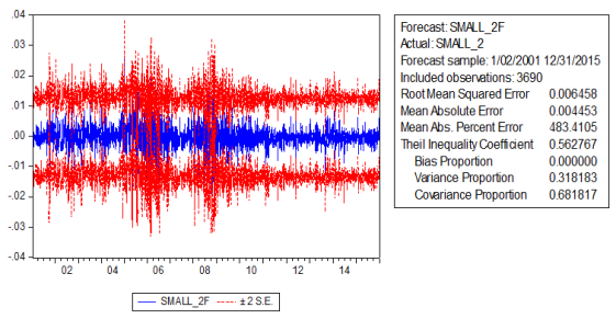
SMALL 2	-0.0003***	0.425***	-0.026*	0.001	-3.11	35.01	-1.93	0.14	26.7%	448.78	1.913
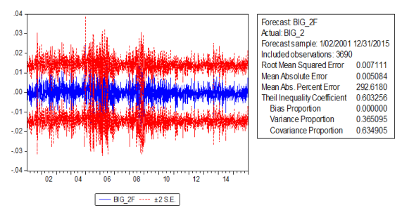
BIG 2	-0.0003**	0.423***	0.018	0.088***	-2.24	31.66	1.25	7.77	21.6%	339.15	1.842
BIG 1	-0.0002**	0.565***	0.110***	0.350***	-2.02	42.81	7.53	31.40	38.4%	766.69	1.873
BIG	-0.0002	0.547***	0.426***	0.301***	-1.63	35.56	25.01	23.14	32.8%	601.56	1.947

*** Significant different from zero at the 1% level. ** Significant different from zero at the 5% level. * Significant different from zero at the 10% level.

Table 7. The Estimation Result of the FF3F According to Value.

Portfolios	α_i	β_MRP	β_HML	β_SMB	t(α_i)	t(β_MRP)	t(β_HML)	t(β_SMB)	Adjusted R²	F-Ratio	D-W stat
HIGH	-0.0003***	0.703***	0.524***	0.166***	-3.16	56.44	38.01	15.80	52.3%	1349.49	1.907
HIGH 1	-0.0003***	0.538***	0.485***	0.038***	-2.80	43.48	35.35	3.68	43.4%	944.63	1.961
HIGH 2	-0.0002	0.473***	0.043***	0.040***	-1.34	36.41	3.01	3.60	26.9%	453.84	1.987
LOW 2	-0.0001	0.532***	0.038***	0.024**	-1.28	42.66	2.78	2.25	34.0%	634.10	1.798
LOW 1	-0.0003***	0.656***	-0.365***	0.068***	-2.86	53.96	-27.11	6.61	53.4%	1410.45	1.983
LOW	-0.0003**	0.577***	-0.564***	0.134***	-2.21	42.83	-37.81	11.78	51.6%	1310.09	1.862

*** Significant different from zero at the 1% level. ** Significant different from zeroat the 5% level. * Significant different from zero at the 10% level.

Download: Download full-size image

Figure 3. Forecast for Big Size Portfolio.

Download: Download full-size image

Figure 4. Forecast for Small Size Portfolio.

Download: Download full-size image

Figure 5. Forecast for High Value Portfolio.

Download: Download full-size image

Figure 6. Forecast for Low Value Portfolio.

7. Conclusion

This paper set out to forecast asset covariances and variances using multi-scale risk models, employing data from 61 firms listed on the Amman Stock Exchange (ASE) over the period 2001 –2015. By incorporating multi-scale factor structures and variance–covariance modeling techniques, the analysis demonstrated that these models provide reliable and robust predictions of asset risk and return dynamics within the Jordanian capital market.

To ensure robustness, several diagnostic tests, namely the CUSUM test for structural stability, the Granger causality test for predictive relationships, and the unit root test for stationarity—were applied. These diagnostics confirmed both the stability of the dataset and the validity of the estimation approach.

Empirical findings revealed that market risk premium coefficients significantly explain variations in portfolio returns. Moreover, portfolios with lower value stocks consistently outperformed higher value portfolios, while smaller-sized portfolios achieved superior returns compared to their larger counterparts. The statistically significant interceptions across most models indicate their strong explanatory power, with the exception of the BIG, HIGH 2, and LOW 2 portfolios, where limited explanatory significance was observed.

Overall, the findings affirm that multi-scale risk models are appropriate and effective for forecasting both variance and covariance structures. These models capture the complex dynamics of daily portfolio returns in the ASE, offering valuable implications for investors, financial analysts, and policymakers. By improving the understanding of risk and return interrelations, this paper contributes to enhancing portfolio optimization strategies and advancing financial decision-making within emerging markets.

Abbreviations

ASE	Amman Stock Exchange
CAPM	Capital Asset Pricing Model
FF3F	Fama and French Three-factor Model
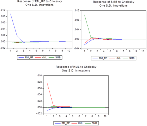
SMB	Small Minus Big (Size Risk Premium)
HML	High Minus Low (Value Risk Premium)
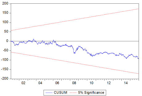
CUSUM	Cumulative Sum Test
ADF	Augmented Dickey-fuller Test

Conflicts of Interest

The authors declare no conflicts of interest.

References

[1]	Abbas, N., Khan, J., Aziz, R., & Sumrani, Z. (2014). A paper to check the applicability of Fama and French three-factor model on KSE 100-Index (2004–2014). International Journal of Financial Research, 6(1), 90.
[2]	Acerbi, C., & Simonetti, P. (2002). Portfolio optimization with spectral measures of risk. arXiv preprint cond-mat/0203607. Retrieved from http://citeseerx.ist.psu.edu/viewdoc/download?doi=10.1.1.311.9257&rep=rep1&type=pdf
[3]	Ajlouni, M. M., Alrabadi, D. W., & Alnader, T. K. (2013). Forecasting the ability of dynamic versus static CAPM: Evidence from Amman Stock Exchange. Jordan Journal of Business Administration, 9(2), 431–443.
[4]	Ajlouni, M. M., & Khasawneh, M. (2017). Empirical test of Fama and French three-factor model in Amman Stock Exchange. Proceedings of the 6th Eurasian Multidisciplinary Forum (EMF 2017), Vienna, Austria, April 27–28.
[5]	Al-Mwalla, M. (2012). Can book-to-market, size, and momentum be extra risk factors that explain the stocks’ rate of return? Evidence from an emerging market. Journal of Finance, Accounting and Management, 3(2), 42–57.
[6]	Al-Mwalla, M., & Karasneh, M. (2011). Fama and French three-factor model: Evidence from an emerging market. European Journal of Economics, Finance and Administrative Sciences, 41, 132–140.
[7]	Ángel Martín Mato, M. (2005). Classic and modern measures of risk in fixed-income portfolio optimization. The Journal of Risk Finance, 6(5), 416–423.
[8]	Berger, T., & Fieberg, C. (2016). On portfolio optimization: Forecasting asset covariances and variances based on multi-scale risk models. The Journal of Risk Finance, 17(3), 295–309.
[9]	Blanco, B. (2012). The use of CAPM and Fama and French three-factor model in portfolio selection. Public and Municipal Finance, 1(2), 62–63.
[10]	Buraschi, A., Porchia, P., & Trojani, F. (2010). Correlation risk and optimal portfolio choice. The Journal of Finance, 65(1), 393–420.
[11]	Chan, L., Karceski, J., & Lakonishok, J. (1999). On portfolio optimization: Forecasting covariances and choosing the risk model. Review of Financial Studies, 12(5), 937–974.
[12]	Chau Li, W., Wu, Y., & Ojiako, U. (2014). Using portfolio optimization models to enhance decision-making and prediction. Journal of Modelling in Management, 9(1), 36–57.
[13]	Da, Z., & Schaumburg, E. (2011). The pricing of volatility risks across asset classes. University of Notre Dame and Federal Reserve Bank of New York (Working Paper).
[14]	Da, Z. (2009). Cash flow, consumption risk, and the cross-section of stock returns. The Journal of Finance, 7(2), 923–956.
[15]	Engles, M. (2004). Portfolio optimization: Beyond Markowitz (master’s thesis). Leiden University.
[16]	Eraslan, V. (2013). Fama and French three-factor model: Evidence from Istanbul Stock Exchange. Business and Economics Research Journal, 4(2), 11–22.
[17]	Fabozzi, F., Gupta, F., & Markowitz, H. (2002). The legacy of modern portfolio theory. The Journal of Investing, 11(3), 7–22.
[18]	Fama, E. F., & French, K. R. (1992). The cross-section of expected stock returns. Journal of Finance, 47(2), 427–465.
[19]	Fama, E. F., & French, K. R. (1993). Common risk factors in the returns on stocks and bonds. Journal of Financial Economics, 33(1), 3–56.
[20]	Fama, E. F., & French, K. R. (1996). Multifactor explanations of asset pricing anomalies. The Journal of Finance, 51(1), 55–84.
[21]	Fama, E. F., & French, K. R. (2014). A five-factor asset pricing model. Journal of Financial Economics, 116(1), 1–22.
[22]	Fama, E. F., & MacBeth, J. D. (1974). Tests of the multiperiod two-parameter model. Journal of Financial Economics, 1(1), 43–66.
[23]	Gençay, R., Whitcher, B., & Selçuk, F. (2003). Systematic risk and time scales. Quantitative Finance, 3(2), 108–116.
[24]	Haugen, A. S. (2001). Modern investment theory (5th ed.). Prentice-Hall.
[25]	Ismal, R. (2014). An optimal risk–return portfolio of Islamic banks. Humanomics, 30(4), 286–303.
[26]	Kaplan, P. D. (1998). Asset allocation models using the Markowitz approach. In Frontiers of Modern Asset Allocation (pp. 267–274).
[27]	Karolyi, G. A., & Wu, Y. (2012). The role of investing ability restrictions on size, value, and momentum in international stock returns. Johnson School Research Paper Series (12-2012).
[28]	Kim, S., & In, F. (2007). A note on the relationship between Fama-French risk factors and innovations of ICAPM state variables. Finance Research Letters, 4(3), 165–171.
[29]	Krokhmal, P., Palmquist, J., & Uryasev, S. (2002). Portfolio optimization with conditional value-at-risk objective and constraints. Journal of Risk, 4, 43–68.
[30]	Li, S., Luong, C., Angkola, F., & Wu, Y. H. (2016). Optimal asset portfolio with stochastic volatility under the mean-variance utility with state-dependent risk aversion. Journal of Industrial and Management Optimization, 12(4), 1521–1533.
[31]	Lintner, J. (1965). The valuation of risk assets and the selection of risky investments in stock portfolios and capital budgets. The Review of Economics and Statistics, 47(1), 13–37.
[32]	Markowitz, H. (1959). Portfolio selection: Efficient diversification of investments. Basil Blackwell.
[33]	Markowitz, H. M. (1952). Portfolio selection. The Journal of Finance, 7(1), 77–91.
[34]	Miller, M. H., & Scholes, M. (1972). Rates of return in relation to risk: A reexamination of some recent findings. In Studies in the Theory of Capital Markets (Vol. 23, pp. 47–78).
[35]	Mossin, J. (1966). Equilibrium in a capital asset market. Econometrica, 98(2), 768–783.
[36]	Patton, A. J., & Timmermann, A. (2010). Monotonicity in asset returns: New tests with applications to the term structure, CAPM, and portfolio sorts. Journal of Financial Economics, 98(3), 605–625.
[37]	Ross, S. A. (1976). The arbitrage theory of capital asset pricing. Journal of Economic Theory, 13(3), 341–360.
[38]	Rotela Junior, P., Pamplona, E. D. O., Rocha, L. C. S., Valerio, V. E. D. M., & Pavia, A. P. (2015). Stochastic portfolio optimization using efficiency evaluation. Management Decision, 53(8), 1698–1713.
[39]	Sharpe, W. F. (1964). Capital asset prices: A theory of market equilibrium under conditions of risk. The Journal of Finance, 19(3), 425–442.
[40]	Sun, Y., Aw, G., Teo, K. L., & Zhou, G. (2015). Portfolio optimization using a new probabilistic risk measure. Journal of Industrial and Management Optimization, 11(4), 1275–1283.
[41]	Treynor, J. L. (1961). Market value, time, and risk. Unpublished manuscript. London: Risk Books.
[42]	Treynor, J. L. (1962). Toward a theory of market value of risky assets. Unpublished manuscript. London: Risk Books.
[43]	Trimech, A., Kortas, H., Benammou, S., & Benammou, S. (2009). Multiscale Fama–French model: Application to the French market. The Journal of Risk Finance, 10(2), 179–192.
[44]	Amman Stock Exchange (ASE). (n.d.). Amman Stock Exchange (official website). Retrieved February 20, 2026, from https://www.ase.com.jo/
[45]	Central Bank of Jordan (CBJ). (n.d.). Central Bank of Jordan (official website). Retrieved February 20, 2026, from https://www.cbj.gov.jo/

Cite This Article

Plain Text BibTeX RIS

APA Style

Hallaq, S. S. A., Ajlouni, M., Alfoul, L. A. (2026). Forecasting Asset Covariances and Variances Using Multi-scale Risk Models: Evidence from the Amman Stock Exchange. Journal of Business and Economic Development, 11(1), 1-15. https://doi.org/10.11648/j.jbed.20261101.11

Copy | Download

ACS Style

Hallaq, S. S. A.; Ajlouni, M.; Alfoul, L. A. Forecasting Asset Covariances and Variances Using Multi-scale Risk Models: Evidence from the Amman Stock Exchange. J. Bus. Econ. Dev. 2026, 11(1), 1-15. doi: 10.11648/j.jbed.20261101.11

Copy | Download

AMA Style

Hallaq SSA, Ajlouni M, Alfoul LA. Forecasting Asset Covariances and Variances Using Multi-scale Risk Models: Evidence from the Amman Stock Exchange. J Bus Econ Dev. 2026;11(1):1-15. doi: 10.11648/j.jbed.20261101.11

Copy | Download

@article{10.11648/j.jbed.20261101.11,
  author = {Said Sami Al Hallaq and Mohammad Ajlouni and Laith Abu- Alfoul},
  title = {Forecasting Asset Covariances and Variances Using 
Multi-scale Risk Models: Evidence from the Amman Stock Exchange},
  journal = {Journal of Business and Economic Development},
  volume = {11},
  number = {1},
  pages = {1-15},
  doi = {10.11648/j.jbed.20261101.11},
  url = {https://doi.org/10.11648/j.jbed.20261101.11},
  eprint = {https://article.sciencepublishinggroup.com/pdf/10.11648.j.jbed.20261101.11},
  abstract = {This study aims to forecast asset variances and covariances through the application of multi-scale risk models. Using daily data for 61 firms listed on the Amman Stock Exchange (ASE) over the period from January 1, 2001, to December 31, 2015, the analysis investigates the dynamic behaviour of asset returns across different time horizons. To enhance the robustness and reliability of the findings, several econometric and statistical techniques are employed, including the CUSUM test to assess structural stability, the Granger causality test to examine predictive relationships, wavelet transformation to capture time-frequency dynamics, and unit root tests to verify stationarity properties. The multi-scale risk model serves as the principal analytical framework, allowing for a comprehensive examination of the evolving interdependencies among asset returns. The empirical results indicate that market risk premium coefficients significantly explain variations in portfolio returns, highlighting the importance of systematic risk factors in asset pricing. Furthermore, portfolios composed of lower-value stocks outperform those containing higher-value stocks, while smaller-sized portfolios consistently generate higher returns than larger-sized portfolios during the sample period. Overall, the findings demonstrate the effectiveness of multi-scale risk models in forecasting asset variances and covariances. The model exhibits strong explanatory power in capturing daily portfolio return dynamics on the ASE, thereby contributing to improved portfolio optimization strategies and more accurate risk prediction. These results underscore the practical and theoretical value of multi-scale modelling in financial risk management.},
 year = {2026}
}

Copy | Download

TY  - JOUR
T1  - Forecasting Asset Covariances and Variances Using 
Multi-scale Risk Models: Evidence from the Amman Stock Exchange
AU  - Said Sami Al Hallaq
AU  - Mohammad Ajlouni
AU  - Laith Abu- Alfoul
Y1  - 2026/02/28
PY  - 2026
N1  - https://doi.org/10.11648/j.jbed.20261101.11
DO  - 10.11648/j.jbed.20261101.11
T2  - Journal of Business and Economic Development
JF  - Journal of Business and Economic Development
JO  - Journal of Business and Economic Development
SP  - 1
EP  - 15
PB  - Science Publishing Group
SN  - 2637-3874
UR  - https://doi.org/10.11648/j.jbed.20261101.11
AB  - This study aims to forecast asset variances and covariances through the application of multi-scale risk models. Using daily data for 61 firms listed on the Amman Stock Exchange (ASE) over the period from January 1, 2001, to December 31, 2015, the analysis investigates the dynamic behaviour of asset returns across different time horizons. To enhance the robustness and reliability of the findings, several econometric and statistical techniques are employed, including the CUSUM test to assess structural stability, the Granger causality test to examine predictive relationships, wavelet transformation to capture time-frequency dynamics, and unit root tests to verify stationarity properties. The multi-scale risk model serves as the principal analytical framework, allowing for a comprehensive examination of the evolving interdependencies among asset returns. The empirical results indicate that market risk premium coefficients significantly explain variations in portfolio returns, highlighting the importance of systematic risk factors in asset pricing. Furthermore, portfolios composed of lower-value stocks outperform those containing higher-value stocks, while smaller-sized portfolios consistently generate higher returns than larger-sized portfolios during the sample period. Overall, the findings demonstrate the effectiveness of multi-scale risk models in forecasting asset variances and covariances. The model exhibits strong explanatory power in capturing daily portfolio return dynamics on the ASE, thereby contributing to improved portfolio optimization strategies and more accurate risk prediction. These results underscore the practical and theoretical value of multi-scale modelling in financial risk management.
VL  - 11
IS  - 1
ER  -

Copy | Download

Author Information

Said Sami Al Hallaq

Department of Business Economics, Yarmouk University, Irbid, Hashemite Kingdom of Jordan

Contact Email

http://orcid.org/0000-0002-5578-5824
Mohammad Ajlouni

Department of Finance, Yarmouk University, Irbid, Hashemite Kingdom of Jordan
Laith Abu- Alfoul

Cairo Amman Bank, Amman, Hashemite Kingdom of Jordan

http://orcid.org/0009-0001-5637-5325

Download PDF

Submit an Article

Plain Text BibTeX RIS

APA Style

Hallaq, S. S. A., Ajlouni, M., Alfoul, L. A. (2026). Forecasting Asset Covariances and Variances Using Multi-scale Risk Models: Evidence from the Amman Stock Exchange. Journal of Business and Economic Development, 11(1), 1-15. https://doi.org/10.11648/j.jbed.20261101.11

Copy | Download

ACS Style

Hallaq, S. S. A.; Ajlouni, M.; Alfoul, L. A. Forecasting Asset Covariances and Variances Using Multi-scale Risk Models: Evidence from the Amman Stock Exchange. J. Bus. Econ. Dev. 2026, 11(1), 1-15. doi: 10.11648/j.jbed.20261101.11

Copy | Download

AMA Style

Hallaq SSA, Ajlouni M, Alfoul LA. Forecasting Asset Covariances and Variances Using Multi-scale Risk Models: Evidence from the Amman Stock Exchange. J Bus Econ Dev. 2026;11(1):1-15. doi: 10.11648/j.jbed.20261101.11

Copy | Download

@article{10.11648/j.jbed.20261101.11,
  author = {Said Sami Al Hallaq and Mohammad Ajlouni and Laith Abu- Alfoul},
  title = {Forecasting Asset Covariances and Variances Using 
Multi-scale Risk Models: Evidence from the Amman Stock Exchange},
  journal = {Journal of Business and Economic Development},
  volume = {11},
  number = {1},
  pages = {1-15},
  doi = {10.11648/j.jbed.20261101.11},
  url = {https://doi.org/10.11648/j.jbed.20261101.11},
  eprint = {https://article.sciencepublishinggroup.com/pdf/10.11648.j.jbed.20261101.11},
  abstract = {This study aims to forecast asset variances and covariances through the application of multi-scale risk models. Using daily data for 61 firms listed on the Amman Stock Exchange (ASE) over the period from January 1, 2001, to December 31, 2015, the analysis investigates the dynamic behaviour of asset returns across different time horizons. To enhance the robustness and reliability of the findings, several econometric and statistical techniques are employed, including the CUSUM test to assess structural stability, the Granger causality test to examine predictive relationships, wavelet transformation to capture time-frequency dynamics, and unit root tests to verify stationarity properties. The multi-scale risk model serves as the principal analytical framework, allowing for a comprehensive examination of the evolving interdependencies among asset returns. The empirical results indicate that market risk premium coefficients significantly explain variations in portfolio returns, highlighting the importance of systematic risk factors in asset pricing. Furthermore, portfolios composed of lower-value stocks outperform those containing higher-value stocks, while smaller-sized portfolios consistently generate higher returns than larger-sized portfolios during the sample period. Overall, the findings demonstrate the effectiveness of multi-scale risk models in forecasting asset variances and covariances. The model exhibits strong explanatory power in capturing daily portfolio return dynamics on the ASE, thereby contributing to improved portfolio optimization strategies and more accurate risk prediction. These results underscore the practical and theoretical value of multi-scale modelling in financial risk management.},
 year = {2026}
}

Copy | Download

TY  - JOUR
T1  - Forecasting Asset Covariances and Variances Using 
Multi-scale Risk Models: Evidence from the Amman Stock Exchange
AU  - Said Sami Al Hallaq
AU  - Mohammad Ajlouni
AU  - Laith Abu- Alfoul
Y1  - 2026/02/28
PY  - 2026
N1  - https://doi.org/10.11648/j.jbed.20261101.11
DO  - 10.11648/j.jbed.20261101.11
T2  - Journal of Business and Economic Development
JF  - Journal of Business and Economic Development
JO  - Journal of Business and Economic Development
SP  - 1
EP  - 15
PB  - Science Publishing Group
SN  - 2637-3874
UR  - https://doi.org/10.11648/j.jbed.20261101.11
AB  - This study aims to forecast asset variances and covariances through the application of multi-scale risk models. Using daily data for 61 firms listed on the Amman Stock Exchange (ASE) over the period from January 1, 2001, to December 31, 2015, the analysis investigates the dynamic behaviour of asset returns across different time horizons. To enhance the robustness and reliability of the findings, several econometric and statistical techniques are employed, including the CUSUM test to assess structural stability, the Granger causality test to examine predictive relationships, wavelet transformation to capture time-frequency dynamics, and unit root tests to verify stationarity properties. The multi-scale risk model serves as the principal analytical framework, allowing for a comprehensive examination of the evolving interdependencies among asset returns. The empirical results indicate that market risk premium coefficients significantly explain variations in portfolio returns, highlighting the importance of systematic risk factors in asset pricing. Furthermore, portfolios composed of lower-value stocks outperform those containing higher-value stocks, while smaller-sized portfolios consistently generate higher returns than larger-sized portfolios during the sample period. Overall, the findings demonstrate the effectiveness of multi-scale risk models in forecasting asset variances and covariances. The model exhibits strong explanatory power in capturing daily portfolio return dynamics on the ASE, thereby contributing to improved portfolio optimization strategies and more accurate risk prediction. These results underscore the practical and theoretical value of multi-scale modelling in financial risk management.
VL  - 11
IS  - 1
ER  -

Copy | Download